This article picks up where the previous one left off. If you have not read the antecedent article on choosing the right prediction horizon, start here: https://x.com/structure_fi/status/2052441182936965191

Once you have chosen a forecast horizon, the next question is feature engineering.

The horizon-selection step answers: what future return are we trying to predict?

Feature engineering answers: what information might help predict it?

This is where a lot of people get lost. They jump straight from "I want to predict returns" into a giant pile of candidate inputs: market data, wallet flows, funding rates, news, social data, influencer tweets, liquidations, macro series, and whatever else feels like it might matter.

Some of those inputs may matter. Eventually.

But the first place to start is usually much simpler: the market data itself.

Before reaching for exotic data, you should understand what can be extracted from the price, spread, volume, and order-flow series directly in front of you. These are the variables every strategy will see, the variables closest to execution, and the variables least likely to create operational mess before you even know whether the idea has legs.

The goal of feature engineering is not to create as many columns as possible.

The goal is disciplined hypothesis generation.

You are trying to transform raw market data into statistics that might contain predictive information about the target you defined in the previous step. If the target is a future return over some horizon h, then your features should be things that plausibly tell you something about that future return.

Not everything that is interesting is useful.

Not everything that is predictive is tradable.

And not every feature that works in a notebook survives contact with live execution.

That is why I like starting with a very basic family of features: smooth operators applied to tick-wise market data.

Start With Smooth Operators

Raw tick data is noisy.

The mid price jumps around. Trades print irregularly. The top of book flickers. A single update can be microstructure noise rather than information.

If you feed raw ticks directly into a model without thinking, the model may spend most of its effort learning noise.

Smooth operators are a way to compress raw market data into more stable measurements.

A moving average is the simplest example. It asks: what is the recent average level of this series?

A volatility estimate asks: how much has this series been moving recently?

A differential operator asks: how quickly is this series changing right now?

These all belong to the same broader family of moving-average features. They take a noisy stream and apply a smoothing kernel to produce a statistic that is easier to reason about.

The same idea is not limited to price. You can apply smooth operators to spread size, traded volume, log volume, order-flow imbalance, signed trade flow, book depth, funding, liquidation flow, or any other stream that is observable at decision time.

That is the useful abstraction: pick a data stream, pick a kernel shape, and compute a causal statistic.

For a first directional strategy, one of the most useful kernel shapes to understand is a smooth differential operator.

The Smooth Differential Operator

The intuition is simple.

We want a feature that behaves like a local slope.

If the smoothed price now is meaningfully above a slower-memory version of the past, the operator is positive. If the smoothed price now is below that slower-memory version of the past, the operator is negative. If the two are close, the operator is near zero.

You can think of this as a smooth derivative of market data.

You can also think of it as a present-return-like feature: not the future return we are trying to predict, but a compressed measure of what the market is doing now.

The useful version should be causal. It should only use data available up to the current tick. A recursive exponential smoothing kernel gives us that.

There is one practical detail that matters: tick data is not sampled at perfectly regular integer seconds.

Market data arrives at discrete points in time, but those points are stochastic. Sometimes ticks arrive quickly. Sometimes there is a gap. The update rule needs to account for how much time has actually passed since the previous observation.

For a series observed as x_i at event times t_i, define the elapsed time between observations as:

Then an exponential moving average with half-life H_tau uses a time-dependent update weight:

Now compute two smoothed versions of the same series: a fast one and a slow one.

The smooth differential operator is the difference between them, normalized by the effective time separation:

For price data, we can also express the operator in basis points per second:

This is not magic. It is a practical, causal, recursively updated convolution-style operator.

The fast EMA behaves like a smoothed version of "approximately now." The slow EMA behaves like a smoothed version of "approximately some time ago." Their difference gives a local directional measurement.

That measurement can become a feature in a model.

What The Kernel Looks Like

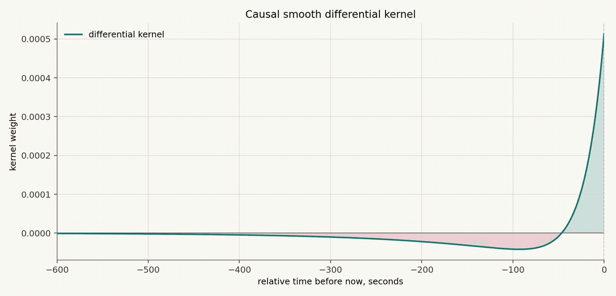
The differential operator can also be understood through its kernel.

The kernel starts positive at the current tick. Looking backward in time, it smoothly decays, crosses below zero, and then approaches zero again from the negative side.

That shape is the whole point.

Recent observations get positive weight. Older observations get negative weight. Very old observations fade away.

That is why the operator behaves like a smooth derivative: it compares the recent present against a smoothed memory of the past.

Other Kernel Shapes

The differential operator is only one kernel shape.

A feature can be written abstractly as a causal weighted average over the past:

Here, x_j is the data stream and k is the kernel. The kernel decides what kind of structure the feature extracts.

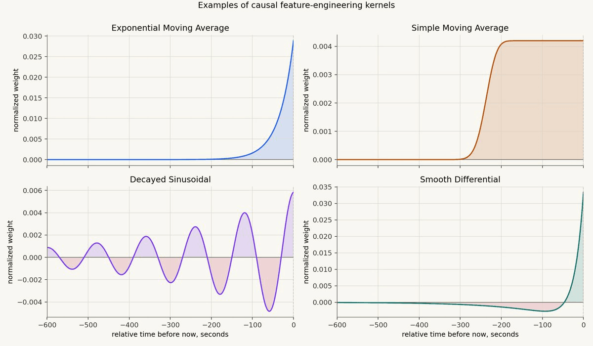
Different kernels ask different questions.

An exponential averaging kernel asks: what is the recent level of this stream?

A differential kernel asks: is the recent present above or below the slower memory of the past?

A sinusoidal kernel asks: does the recent history line up with a cycle at a particular period?

The sinusoidal case is useful when you suspect seasonality, oscillation, mean reversion, or autocorrelative or anticorrelative structure at a specific time scale.

For example, maybe spread widening tends to mean-revert over a few minutes. Maybe volume arrives in bursts with a characteristic rhythm. Maybe the price series has intraday periodicity. A decayed sine/cosine pair lets the model ask whether the recent path has phase and amplitude at that period.

You usually want both sine and cosine features. One captures one phase of the cycle; the other captures the phase shifted by a quarter period. Together, they let the model represent cyclic structure without assuming the turning points line up perfectly with your clock.

A classical windowed moving average asks: what was the average over the last W seconds?

That is a useful idea, but the hard cutoff at the edge of the window can be awkward. A point just inside the window gets full weight. A point just outside the window gets zero. In live tick data, those discontinuities are not always what you want.

A smooth approximation is to average many iterated EMAs. Define tau_prime as:

Then:

The analytical kernel is:

With a large n, this becomes a much more rectangular-looking kernel. The top is nearly flat, and the old edge rolls off smoothly instead of dropping to zero instantly.

This matters because most useful feature families come from combining data streams with kernel shapes.

You might compute a differential operator on mid-price to measure local slope.

You might compute a smooth window on spread to measure whether liquidity has recently deteriorated.

You might compute a sinusoidal operator on volume to measure whether trading intensity has entered a recurring burst pattern.

You might compute an exponential average of order-flow imbalance to measure whether buying or selling pressure has persisted.

This is the feature-engineering mindset.

You are not inventing random columns.

You are choosing a market data stream and a question to ask of its recent history.

Why This Is A Good First Feature Family

The point is not that this exact operator is always predictive.

The point is that it gives you a disciplined starting place.

You can scan many half-lives: 5s, 15s, 30s, 1m, 5m, 15m, 1h, and so on. Each half-life gives the model a different view of market motion. Short operators react quickly. Long operators move slowly but may be less noisy.

But the scan should still be connected to the target horizon.

If your target variable is a future return over several days, it probably does not make much sense to spend most of your search on half-lives measured in seconds. Those features may still matter if you have a specific microstructure hypothesis, but as a default, scanning half-lives that are much smaller than the target horizon mostly increases noise and research degrees of freedom.

The cleaner approach is to search over time scales that plausibly relate to the horizon you are trying to predict.

This turns feature engineering into a structured search instead of a vibes exercise.

You are not asking "what random data can I throw at the model?"

You are asking "which time scales of recent market behavior contain information about the future return target?"

That is a much better question.

And it fits naturally into the strategy research pipeline:

1. Choose the forecast horizon.

2. Define the target variable.

3. Build causal features available at decision time.

4. Train models to predict the target.

5. Validate out of sample with time-aware splits.

6. Convert model output into strategy states and target positions.

Feature engineering is step three.

It is the bridge between raw market data and the predictive model.

Example Data And Operator Plot

For the first illustration, I generated 1,000 synthetic tick observations with stochastic timestamps and a few realistic market-data features:

• clustered volatility

• changing drift

• order-flow pressure

• small random jumps

• transient microstructure noise

• tick-size rounding

The synthetic returns also include a light periodic component, so the sinusoidal feature has a real seasonal pattern to detect without making the raw price path look like a toy sine wave.

The data is intentionally synthetic. The goal is not to imply that this exact path is tradable. The goal is to show how the operator behaves when the market changes character.

The top panel shows the raw mid-price, fast EMA, and slow EMA. The bottom panel shows the smooth differential operator. The x-axes are aligned and measured in seconds.

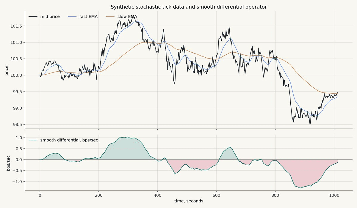
What matters is the alignment between the top and bottom panels.

When the fast EMA rises above the slow EMA, the differential operator turns positive. When price begins to roll over and the fast EMA crosses below the slow EMA, the operator turns negative. When the recovery regime begins, the operator climbs back toward zero and then positive territory.

This is exactly the behavior we want from a first-pass market-data feature.

It is not predicting the future by itself.

It is summarizing the recent local shape of the market in a way a model can use.

Same Data, Three More Kernels

The same tick series can be transformed by the other kernels too.

This is the part that makes the abstraction useful. Once the data stream and timestamp handling are correct, changing the feature is mostly a matter of changing the kernel shape.

In the chart below, the top panel is the same raw mid-price series. The next two panels show price-level transforms: an exponential moving average and a smooth Simple Moving Average. The bottom panel converts the same ticks into returns and applies a decayed sinusoidal detector.

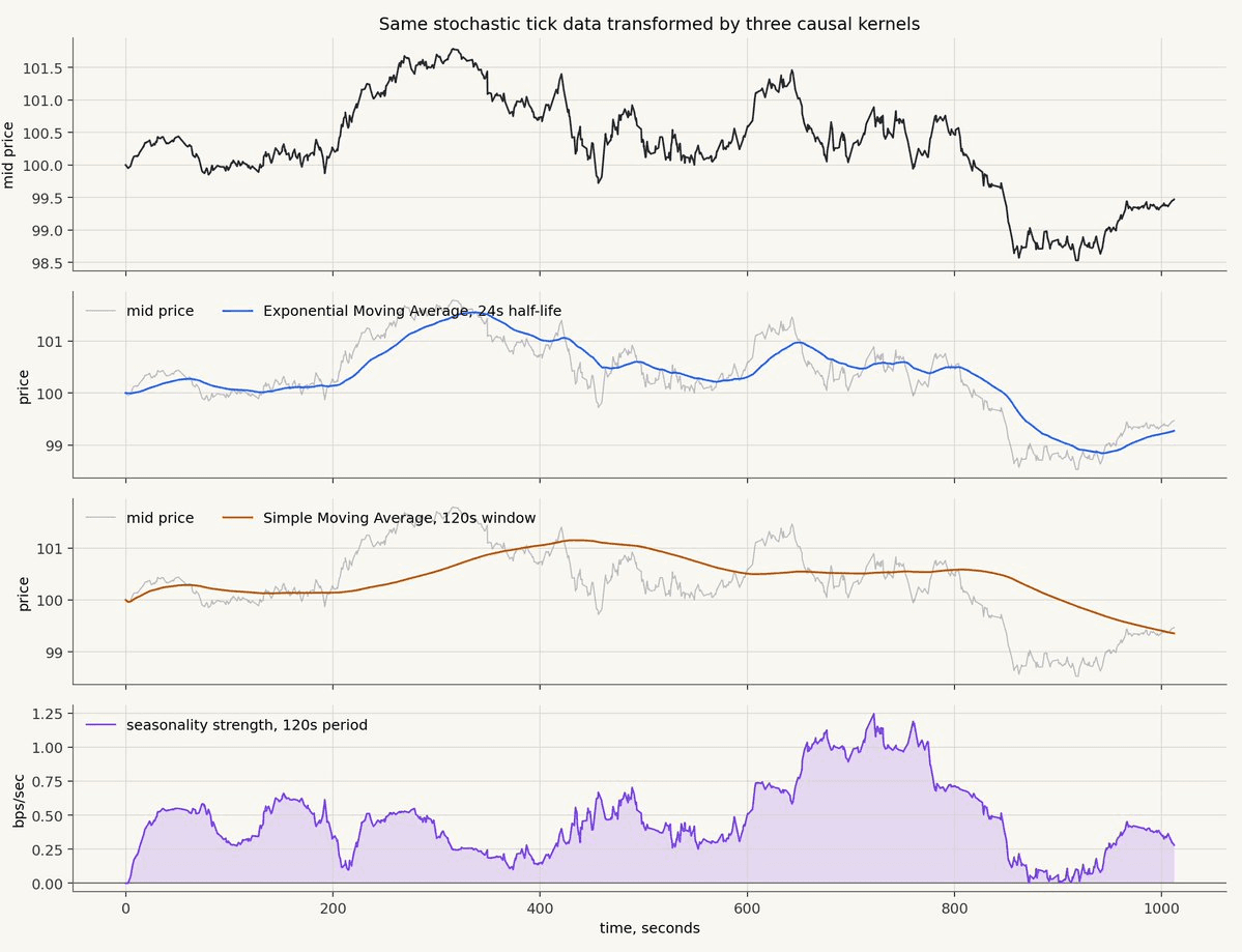
The exponential moving average follows the recent level of the market. It reacts faster than the Simple Moving Average because it puts the most weight on the newest observations and then decays smoothly into the past.

The Simple Moving Average is slower and more level-headed. It acts like a broad trailing window, so it is less interested in the latest tick and more interested in the average state of the market over a recent block of time.

The decayed sinusoidal feature is different. It is not trying to estimate the level of the price. It looks at the tick-to-tick return stream and asks whether recent returns contain energy at a particular period. In this example, the kernel is tuned to the same light seasonal component planted in the synthetic data, so the response rises when that structure becomes easier to detect.

These are three different questions asked of the same data.

What is the recent level?

What is the recent broad average?

Is there cyclic structure at this time scale?

That is feature engineering in its cleanest form.

This Is Enough To Make You Dangerous

With this toolkit, you can start building serious feature sets.

You now have a practical way to transform almost any discrete time series into well-behaved model features. Price, spread, volume, order-flow imbalance, book depth, funding, liquidation flow, signed trade flow: if it is observable at decision time, you can apply causal kernels to it.

The workflow is simple:

1. Choose a data stream.

2. Choose a kernel shape.

3. Choose a time scale that makes sense relative to the target horizon.

4. Compute the feature using only information available at that time.

5. Feed the resulting feature into the modeling step.

This does not mean the feature is predictive.

It means the feature is now well-formed enough to test.

Up next: heuristics for telling whether these features are actually capturing predictive information about the target variable we care about, future returns.

Not Financial Advice

The content above is for general educational and informational purposes only. It is not financial, investment, trading, legal, tax, accounting, or other professional advice, and it is not a recommendation, offer, or solicitation to buy, sell, hold, or use any asset, strategy, protocol, venue, or financial product.

Trading and automated strategies involve substantial risk, including the possible loss of principal. Crypto assets and DeFi markets can be highly volatile, illiquid, technically complex, and subject to execution, smart contract, custody, regulatory, and counterparty risks. Past performance, backtests, simulations, or examples do not guarantee future results.

You are responsible for your own decisions. Do your own research, understand the risks, and consult qualified professional advisers before making financial, legal, tax, or trading decisions. Structure does not provide personalized investment advice and does not guarantee any strategy outcome, return, or level of performance.