From Features To Forecasts: How To Train A Trading Model
Time to read:
15min
This article picks up after the previous post on testing whether a feature has predictive information. If you have not read it yet, start here: https://x.com/structure_fi/status/2054180738363215877
At this point, we have done the work that most people want to skip. We chose a target horizon. We built causal features. We checked conditional behavior. We measured IC, rank IC, nonlinear dependence, incremental value, multiple testing, and basic economic usefulness.
Now comes the part people usually over-romanticize: training the model.
The model is not where you magically find predictive information. The model is where you force useful features to compete under a forecasting objective.
That framing matters. If your features are weak, the model will not save you. If your validation is leaking, the model will flatter you. If your preprocessing uses the future, the model will quietly cheat. And if your model output cannot survive execution, the whole thing is still just a pretty notebook.
The job is narrower and more useful: turn features available at decision time into stable forecasts of a future return target.
In symbols, if x_t is the feature vector at time t, and r_{t,h} is the future return over horizon h, the model is a mapping:
Training chooses the parameters theta by minimizing some loss on historical examples:
That formula looks clean. The real work is in every word around it: what features go into x_t, how they are normalized, what loss ell means, how flexible f_theta is allowed to be, and whether the validation setup resembles the future the model will actually face.
I have seen a version of this mistake many times: someone spends weeks testing model classes when the real bug was a z-score computed on the full dataset. The model was not brilliant. It had been handed a little information from the future.
So before choosing the fancy model, get the boring parts right.
(It's amazing how in systematic trading, as in so many other disciplines, the ability to get the boring details right, consistently, is what separates unbelievable success from mediocrity or ruin.)
Start With The Baseline
Every modeling project needs a baseline that is almost embarrassingly simple.
That might be:
predict zero
predict the recent historical mean
predict a simple momentum or reversal signal
fit a linear model on a few core features
use the current production or research model
The baseline is not there to impress anyone. It is there to keep you honest.
If a complex model cannot beat a simple baseline out of sample, the complex model is not useful yet. It might become useful after better features, better normalization, or a better loss function. But at that moment, the model has not earned its complexity.
This is one of those lessons that feels too basic until you watch a complicated research stack lose to a regularized linear model. At trading firms, that is not a theoretical embarrassment. It happens. The market is noisy, samples are smaller than they look, and flexible models are very good at memorizing yesterday's weirdness.
Suppose the baseline forecast is \hat r^{(0)}_{t,h} and the challenger forecast is \hat r^{(1)}_{t,h}. The comparison should be made on the same out-of-sample timestamps:
The challenger only matters if its errors are better in a way that survives the validation discipline from the previous post.
Normalize Features Without Cheating
Most model classes behave badly when features have incompatible scales. A feature measured in basis points, a spread measured in ticks, a volume feature measured in dollars, and a funding feature measured in annualized percent should not be thrown into the same model raw unless the model class is explicitly robust to that.
The common choices are:
z-score normalization
causal rolling z-score normalization
rank or percentile transforms
winsorization or clipping
robust scaling by median and MAD
volatility normalization
per-asset normalization for cross-sectional models
The dangerous version is full-sample normalization.
If you compute the mean and standard deviation using the entire dataset, the future has influenced the feature. Even if the return label is not used, the transformation still knows about future regimes. That can be enough to make a model look cleaner than it would have been live.
The non-leaking version fits normalization on the training period or computes it causally through time.
For a causal z-score, maintain a rolling or exponentially weighted mean and variance:
Then normalize using only information available up to time t:
In production, you would usually add small numerical guards, clipping, and warmup logic. The principle is the important part: no future rows.
The chart below shows why this matters. The raw feature changes level and volatility after the validation regime begins. The full-sample z-score already knows about that later regime. The causal z-score adapts only after the shift occurs.
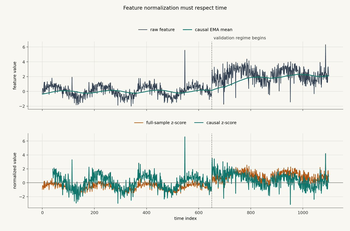
This is a small synthetic example, but the failure mode is real. After major volatility shocks, models trained on calm data often discover that their idea of "normal" was not normal at all. A full-sample scaler hides that lesson. A causal scaler makes you live through it.
Rank transforms are another useful tool. Instead of preserving the raw magnitude, convert a feature into a percentile score relative to recent history:
This can make heavy-tailed features easier to model. It can also stabilize features across assets. The tradeoff is that ranks throw away magnitude. Sometimes that is good. Sometimes the magnitude is the point.
Winsorization and clipping are similarly practical. If one liquidation event or one bad print can dominate a feature, a model may learn the event instead of the relationship. A clipped feature says: beyond this point, I care that the value is extreme, but I do not want the exact size of the extreme to control the fit.
Linearize What You Can
A linear model does not require raw linear features.
This is one of the most useful tricks in practical modeling. If the relationship has shape, you can often transform the feature so a simple model can learn it.
Suppose a feature only matters in the tails. The raw feature x_t may not be enough. You can add tail transforms:
Then a linear model can treat the middle and tails differently:
You can do the same with bucket indicators, splines, signed log transforms, volatility-scaled features, interactions, and monotonic transforms.
This is not cheating. It is feature engineering for the model class.
The chart below shows a synthetic feature where the tails matter more than the middle. A raw linear fit sees the broad direction, but it misses the change in slope. A linear model with a tail transform can express the relationship without becoming a black box.
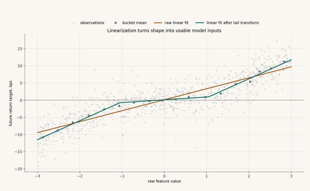
This is often the highest-return modeling work. Before reaching for a larger model, ask whether a simple transformation would make the relationship obvious.
There is a personal reason I like this step. When a model is wrong, you need to debug it. A transformed linear feature is easier to inspect than a flexible model that discovered the same shape in a hidden way. You can look at the coefficient, bucket the transformed feature, and ask whether the behavior makes sense.
The Main Model Families
Once the features are normalized and shaped, the model class becomes a more meaningful choice.
The model class is not just an implementation detail. It is an assumption about the shape of the relationship.
Linear Models:
Linear models assume the forecast is an additive combination of features:
The basic version is ordinary least squares. In trading research, the more useful versions are usually regularized:
Ridge shrinks coefficients toward zero. Lasso can push some coefficients exactly to zero. Elastic net combines both.
Linear models are not fashionable, but they are hard to beat when the signal-to-noise ratio is low. They are fast, stable, inspectable, and easy to monitor. If a feature only works inside a massive nonlinear model, it may still be real, but it is harder to trust.
For direction classification, logistic regression is the same idea with a probability output:
Tree Models And Boosting:
Tree models learn thresholds.
That makes them useful when the relationship is conditional: spread only matters when volatility is high, momentum only matters when liquidity is thin, or order-flow imbalance only matters after a large move.
A simple tree partitions feature space into regions and assigns each region a prediction:
Boosting combines many weak trees:
Gradient boosted trees often perform well on tabular data because they learn thresholds and interactions without requiring you to specify every interaction by hand.
The risk is that they also learn research artifacts. They can split on regime quirks, exchange-specific weirdness, stale features, and subtle leaks. Feature importance can look scientific while hiding unstable dependence.
Neural Nets And Sequence Models:
Neural nets are flexible function approximators:
For engineered tabular features, a small MLP may be enough if you have a lot of data and strong regularization. MLP means multilayer perceptron, which is the standard feedforward neural network: stacked layers of weighted sums and nonlinear activations. For raw sequences, people look at temporal convolutions, recurrent models, transformers, and representation learning.
The caution is simple: flexibility is expensive. You pay in data requirements, validation complexity, monitoring difficulty, and overfitting risk.
There are places where sequence models make sense. If the path itself matters, not just the current feature snapshot, a sequence model may be the right tool. But most trading teams should earn that complexity. Start with models you can debug.
Regime And State Models:
Sometimes the problem is not that the model is too simple. Sometimes the market is in different states.
A model that works during high-liquidity calm markets may fail during liquidation cascades. A feature that predicts short-term continuation during one regime may predict reversal in another.
One way to handle this is to condition the forecast on a regime state s_t:
Another is a mixture-of-experts model:
The regime state might come from volatility, spread, volume, funding, inventory, time of day, market stress, or a learned classifier.
In Structure terms, this is also where the connection to strategy architecture becomes natural. The model output is a signal. Signals can drive state transitions. States resolve to target positions. The execution layer should remain deterministic and auditable.
The forecast is not the strategy. It is one input into the strategy.
Compare Model Shapes Directly
The chart below shows the same synthetic training data fit with three model classes: a linear model, a piecewise linear model, and a tree-like bucket model. The true relationship is hidden from the model, but shown in black for illustration.
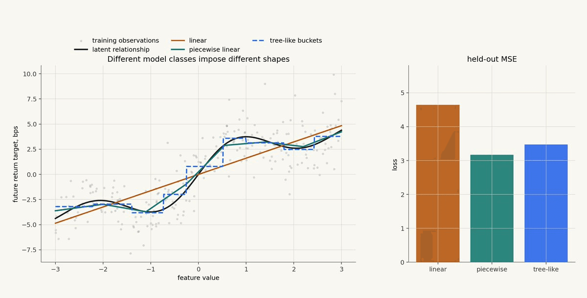
The linear model is stable but too rigid. The tree-like model captures thresholds but creates step changes. The piecewise linear model captures the broad nonlinear shape while staying relatively smooth.
This is one practical use of synthetic data. When you know the right answer, you can test whether your model fitting pipeline can recover it. You can see whether the model underfits, overfits, invents thresholds, extrapolates wildly, or behaves sensibly when the data gets noisy.
That is not a substitute for real market validation. It is a calibration tool for your own research process. If your code cannot recover a simple known relationship in synthetic data, it is probably not ready to interpret a messy market relationship where the truth is hidden.
You should also inspect what the model says outside the range of training data. This matters for both the input features and the target forecast. If the model only trained on feature values between -3 and 3, what happens when live data prints 8? Does the prediction saturate? Does it stay conservative? Or does it explode into a huge target return estimate because the model extrapolated a curve it barely understood?
That kind of blowup can be dangerous. An extreme outlier in the input features should not automatically create an extreme target prediction. Often the better behavior is to say: this observation is far outside the training distribution, so the model should not make a confident forecast here.
You can handle that directly in the modeling step. Clip or saturate features. Add out-of-distribution flags. Train a separate "unknown regime" state. Set confidence to zero when too many inputs are outside historical ranges. Or route the strategy into a defensive state where it reduces risk or exits until the market looks recognizable again.
When the market enters a regime you have not seen before, sometimes the right forecast is not "up" or "down." Sometimes the right forecast is "I do not know."
This is the tradeoff you are always making.
A model that is too simple can underfit. A model that is too flexible can fit noise. A model that is hard to inspect can work in research and become miserable in production.
The right model is not the most powerful one. It is the simplest model that captures the structure you have evidence for.
Choose The Loss Function
The loss function defines what the model is trying to be good at.
Mean squared error is common for return forecasting:
It punishes large errors heavily. That can be useful if large misses are especially bad, but it also makes the model sensitive to outliers.
Absolute error is more robust:
Huber loss is a compromise. It is quadratic near zero and linear in the tails:
Quantile loss is useful when you care about a conditional quantile instead of the mean:
Ranking losses are useful when the model is mainly used to rank opportunities. Cost-aware losses can include turnover, slippage, fees, and position constraints, but then the assumptions need to be explicit.
The chart below shows the basic shape of squared error, absolute error, and Huber loss.
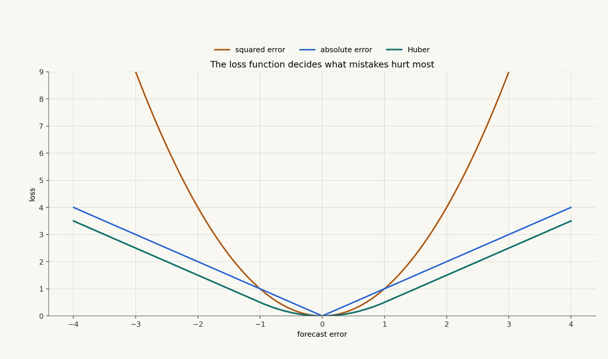
The lesson is not that one loss is always better. The lesson is that loss choice encodes a trading preference. If you care about calibrated expected return, MSE may be reasonable. If you care about robustness, Huber or absolute error may be better. If the model feeds a ranking engine, a ranking objective may match the use case more directly.
The first time you see a model look great under one loss and mediocre under another, do not treat that as a nuisance. It is telling you what the model is actually good at.
Regularization Is Not Optional
Regularization is not a hack. It is an admission that markets are noisy and the effective sample size is smaller than the row count.
The general regularized objective is:
Here, Omega(theta) penalizes complexity. In ridge regression it is the squared coefficient norm. In tree models it can be maximum depth, minimum samples per leaf, shrinkage, feature subsampling, or early stopping. In neural nets it can be weight decay, dropout, architecture limits, and early stopping.
The chart below shows a small synthetic example. As polynomial degree increases, training loss keeps falling. The unregularized test loss eventually explodes. The ridge version gives up some flexibility, but stays controlled.
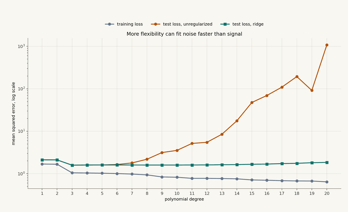
This chart is exaggerated on purpose, but the pattern is familiar. The backtest looks better and better as the model learns more degrees of freedom. Then the next regime arrives and the model discovers it had been memorizing noise.
You can see this after volatility shocks, venue changes, fee changes, and liquidity migrations. The model did not just learn "the market." It learned a sample. Regularization is one way to stop the sample from taking over.
Train Like The Future Is Actually Unknown
The validation rules from the previous post still apply.
Use forward time splits. Train on earlier data and test on later data. If labels overlap, use embargoes so the training set does not sit too close to the test labels. Fit preprocessing only on training data. Tune hyperparameters without touching the final holdout.
For walk-forward training, repeat the process through time:
Then train on D_train and evaluate on the next block D_test.
This is slower than random splitting. Good. Random splitting is often too generous for market data.
One practical scar: if your validation is fast and comfortable, it is worth asking whether it is too easy. Real trading does not shuffle rows. It gives you yesterday, then today, then tomorrow, in order.
Interpret The Forecast Output
A model output is not automatically a trade.
The output might mean:
expected future return
probability of a positive return
rank score
volatility-adjusted score
trade/no-trade score
input into a state machine
If the model outputs an expected return, you still need sizing, risk controls, execution logic, and constraints. A simple educational mapping might look like:
Here, q_t is a target position, k is a scaling parameter, sigma_t is a volatility estimate, and q_max is a position limit.
This is not a universal sizing rule. It is a reminder that forecasts need translation. The model says something about expected return. The strategy has to decide what position, if any, should result.
In a production system, this translation should be inspectable. A signal should be reproducible. A state transition should be explainable. A target position should be auditable. That is how you debug a strategy when the market changes.
A Practical Model Selection Order
If you are starting from engineered features, the most reasonable order is usually:
zero or simple historical baseline
regularized linear model
transformed linear model with splines, tails, ranks, and interactions
tree or boosted-tree model for thresholds and interactions
regime-conditioned model if behavior clearly changes by market state
neural or sequence model only when the data and validation discipline justify it
This order is not about being conservative for its own sake. It is about controlling degrees of freedom.
Every model class adds ways to be right and ways to fool yourself. The goal is to add flexibility only when the evidence says the relationship needs it.
The best modeling work often feels almost boring from the outside. The features are causal. The normalizers are causal. The baseline is clear. The model is regularized. The validation is forward. The output is connected to execution constraints. Nothing is mystical.
That is what makes it useful.
The Point
Training a trading model is not a contest to use the fanciest algorithm.
It is a discipline for converting tested features into stable forecasts.
Normalize without leakage. Linearize the shapes you already understand. Start with baselines. Choose the model class that matches the evidence. Pick a loss function that matches the use case. Regularize harder than your ego wants. Validate like the future is actually unknown. Then translate the forecast into deterministic strategy logic that can be inspected, tested, and executed.
If the feature work was the search for useful information, model training is the pressure test.
The model should not make the research more mysterious.
It should make the assumptions explicit.
Not Financial Advice
The content above is for general educational and informational purposes only. It is not financial, investment, trading, legal, tax, accounting, or other professional advice, and it is not a recommendation, offer, or solicitation to buy, sell, hold, or use any asset, strategy, protocol, venue, or financial product.
Trading and automated strategies involve substantial risk, including the possible loss of principal. Crypto assets and DeFi markets can be highly volatile, illiquid, technically complex, and subject to execution, smart contract, custody, regulatory, and counterparty risks. Past performance, backtests, simulations, or examples do not guarantee future results.
You are responsible for your own decisions. Do your own research, understand the risks, and consult qualified professional advisers before making financial, legal, tax, or trading decisions. Structure does not provide personalized investment advice and does not guarantee any strategy outcome, return, or level of performance.