This article picks up after the previous post on training a model from engineered features. If you have not read it yet, start here: https://x.com/structure_fi/status/2054496353267400814

At this point, we have a forecast.

That is not the same thing as having a strategy.

A model can tell you that a future return looks positive, negative, large, small, noisy, stable, ranked in the top decile, or outside anything it has seen before. None of that answers the operational question that matters in production:

What position should the strategy hold right now?

That translation is where a lot of trading systems get quietly dangerous. The research notebook says +4 bps expected return. The live system needs to decide whether to do nothing, enter, add, reduce, pause, cross the spread, post passively, or get out because the market no longer looks like the one the model was trained on.

The model is a measurement device.

The strategy is a decision system.

This post is about the layer between them: position construction, state, and execution.

It is less glamorous than model training. It is also where many good-looking forecasts turn into bad live behavior.

The first time you see this in a real backtest, it feels annoying. The model looks fine. The conditional buckets look fine. The IC is positive. Then you add costs, thresholds, position caps, latency, and turnover, and the PnL disappears. That is not a small implementation detail. That is the market telling you that the forecast was not yet a tradable policy.

A Forecast Is Not A Position

In the previous step, the model learned a mapping from current information to a future return target:

Here, x_t is the feature vector available at time t, h is the forecast horizon, and r hat is the model's estimate of the future return over that horizon.

The strategy now needs a second mapping:

Here, q_target is the target position, sigma_t is a volatility estimate, c_t is expected cost or frictions, L_t represents limits and constraints, and s_t is the current strategy state.

That second function, g, is where the forecast becomes a trading decision.

It answers questions like:

• Is the forecast large enough to overcome costs?

• Is the market liquid enough to trade?

• How much risk should we take for this forecast?

• Should the strategy enter, add, reduce, or stay flat?

• Are we in a regime where the model is allowed to express risk?

• How quickly should the executor move toward the target?

This is why Structure strategies are built around data, computations, signals, state machines, target positions, and executors. Those pieces are not ceremony. They separate "what do we observe?" from "what do we believe?" from "what do we do?"

Without that separation, a strategy becomes a pile of clever code where the model, risk logic, execution logic, and emergency behavior are all tangled together. That might work for a demo. It is miserable to debug when real money, real latency, and real fills are involved.

Define The Position Function

The simplest bad position function is this:

If the forecast is positive, go long. If the forecast is negative, go short.

That is usually too crude.

Small forecasts are often noise. Medium forecasts may deserve partial exposure. Large forecasts may deserve full exposure, but only up to a cap. And every forecast needs to be compared against costs, slippage, volatility, and risk limits.

A more realistic educational position function has three regions:

• a no-trade zone near zero

• a ramp where position increases with forecast strength

• a cap where the strategy refuses to size larger

One simple version looks like this:

Here, theta_t is the no-trade threshold, a_t controls how quickly the strategy scales in, and q_max is the position cap.

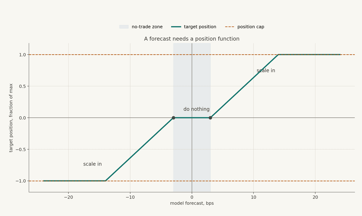
The picture is simple, but the habit is important.

Do not let a model output become a position by accident. Make the translation explicit.

This is one of the lessons people associate with the 1987 crash and portfolio insurance. In the years before Black Monday, large institutions had started using computer-assisted hedging programs that calculated how much stock exposure to hold at different market levels. The basic idea was intuitive: keep upside exposure in rising markets, and reduce exposure as markets fell, often by selling stock-index futures instead of the underlying stocks.

That sounds prudent at the level of a single portfolio. The problem is that markets do not experience one portfolio in isolation. If many large portfolios follow similar rules, and those rules all ask for less exposure as prices fall, the position function itself becomes a source of flow. Selling can push prices lower, lower prices can trigger more selling, and the strategy that looked like insurance in a spreadsheet can become part of a broader feedback loop.

That does not make deterministic rules the villain. Automated trading depends on rules. The more useful lesson is that a position function is not merely an internal implementation detail; it is a behavioral contract with the market. A rule that is sensible for one account can become fragile when liquidity is stressed and many participants are being pushed through similar state transitions at the same time.

So the question is broader than whether the forecast has edge. You also want to know how the position function behaves when the forecast is changing quickly, liquidity is thinning, and other market participants may be trying to make the same adjustment.

Small Forecasts Should Often Do Nothing

The most expensive trade is often the one you did not need to make.

If your model forecasts +0.6 bps, and expected cost is 0.8 bps, the trade is already suspect before you discuss model error. If the forecast is also noisy, the better decision may be no position change at all.

A simple trade condition is:

Here, cost_t is the estimated cost of trading, and m_t is a margin of safety. That margin is not philosophical. It is there because your cost estimate is wrong sometimes, your fill model is wrong sometimes, and the forecast itself is uncertain.

One common production mistake is using the same threshold for entering and exiting. The signal crosses the line, the strategy enters. The signal wiggles back under the line, the strategy exits. A few ticks later, it crosses again. Now the system is paying costs to express noise.

This is where hysteresis helps.

The strategy requires a stronger signal to enter than to stay in. You can also add cooldowns, minimum hold times, or minimum target-position changes before trading.

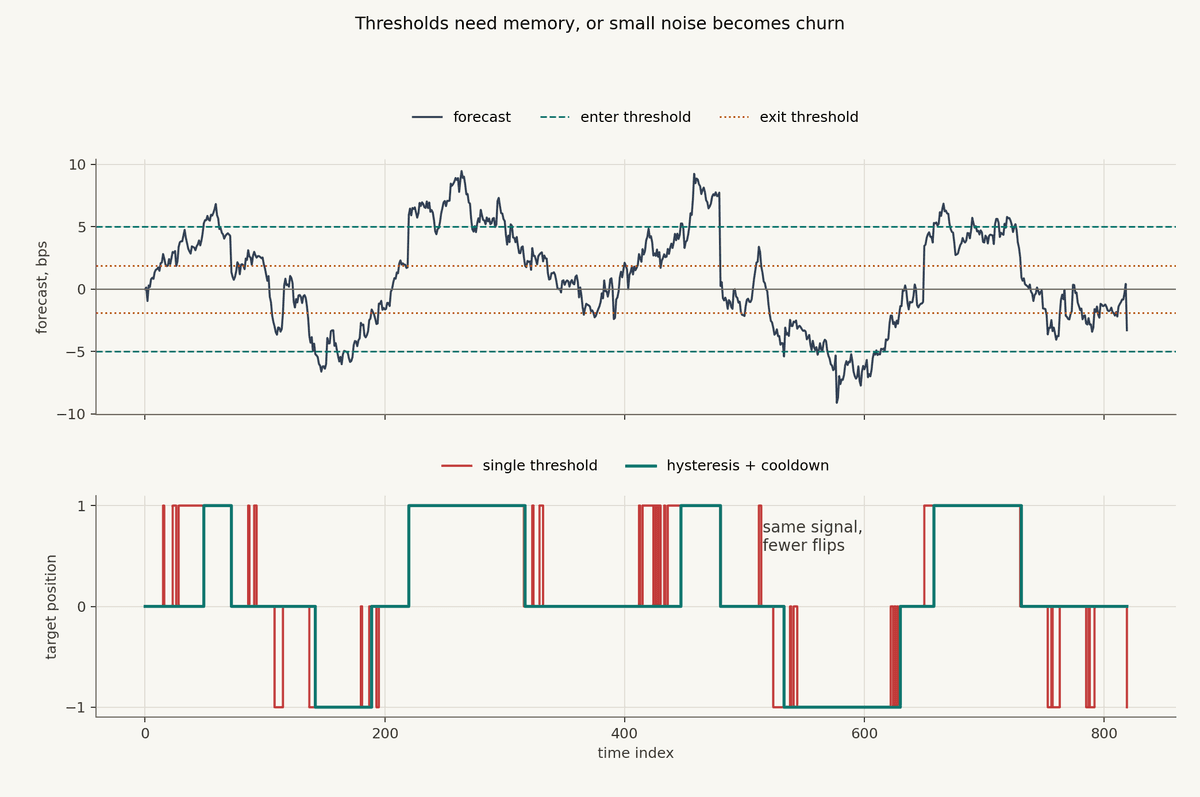
This is not just a fee-saving trick. It changes the personality of the strategy.

A strategy with no memory is twitchy. A strategy with reasonable hysteresis can wait for the signal to matter.

Anyone who has operated automated systems has seen some version of this. The research chart shows a smooth edge. The live blotter shows repeated tiny orders flipping around the best bid and offer, paying spread and fees without enough forecast edge to justify the churn. The bug is not always in the model. Sometimes the bug is that the decision rule treats every tiny forecast update as an instruction to trade.

Size With Risk, Not With Excitement

Forecast magnitude is not the same as trade size.

A 5 bps forecast in a quiet market is not equivalent to a 5 bps forecast in a violent market. The risk, cost, and path dependency are different.

A common educational sizing rule scales expected return by variance:

Then apply caps:

This resembles the intuition behind mean-variance sizing: larger expected return supports more exposure, higher variance supports less exposure. It is not a universal rule. In production, you still need caps, constraints, inventory limits, liquidation awareness, funding awareness, and execution limits.

The practical point is that sizing should be anchored to risk, not excitement.

One of the easiest ways to fool yourself in a backtest is to let position size grow exactly when the market becomes hardest to trade. Volatility spikes, spreads widen, order books thin out, and the naive strategy decides the signal is huge, so it should trade bigger. That can be backwards.

Liquidity is a state variable.

March 2020 was a useful reminder. In the first phase of the COVID shock, Treasuries behaved the way people expect safe assets to behave: risky assets sold off, and Treasury prices initially rose. Then the market flipped into a dash for cash. Investors who needed liquidity sold what they could sell, including Treasuries. Dealers became balance-sheet bottlenecks. A market that normally represents depth and safety suddenly showed severe illiquidity at the same time that stocks were falling.

That episode is worth sitting with because it breaks a lazy assumption. If the U.S. Treasury market can become capacity constrained under stress, then a crypto strategy on permissionless venues should be very careful about treating liquidity as a constant.

A position rule should know how much it is asking the market to absorb:

Here, V_t is a recent volume or capacity estimate, and rho is the maximum fraction of that capacity the strategy is willing to consume.

This is still simplified. Real capacity depends on venue, order type, queue position, volatility, spread, adverse selection, and who else is trying to do the same thing. But even a crude capacity constraint is better than pretending size has no market footprint.

State Machines Make Strategy Logic Inspectable

At this point, the strategy has more than a forecast.

It has thresholds, risk scaling, caps, costs, liquidity limits, and maybe an unknown-regime detector. If you implement all of that as scattered conditionals, you can make it work. You can also make it impossible to reason about.

The cleaner abstraction is a state machine.

The strategy is always in some state: flat, building, risk_on, reducing, paused, unknown_regime, or whatever states match the design. The forecast and market data do not directly spray orders into the world. They update state and target position.

Here, s_t is the strategy state, and ell_t represents liquidity or execution conditions.

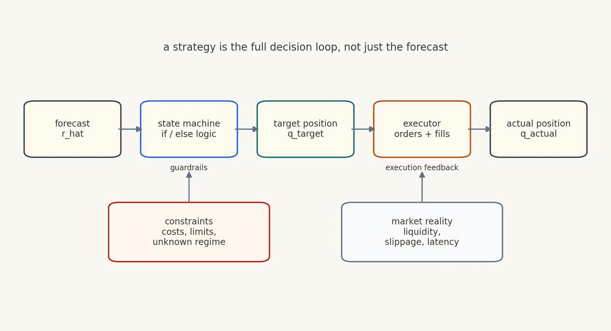
This is where deterministic execution matters.

If a strategy enters unknown_regime, the target position might go to zero. If it enters paused, the executor might stop opening new risk but continue managing existing exposure. If it is building, the executor might move toward the target slowly. If it is risk_on, the strategy might maintain exposure until the exit condition fires.

These distinctions sound small until something breaks.

In a production incident, you do not want to ask, "Why did the model trade?"

You want to ask sharper questions:

• What state was the strategy in?

• What signal caused the transition?

• What target position did the state produce?

• What orders did the executor send?

• What fills actually happened?

• Which version of the strategy logic was running?

This is why auditable logic matters. A model score alone is not enough. You need the decision trail.

The Executor Is Part Of The Strategy

Target position is intent. Actual position is reality.

The executor is the layer that tries to move from one to the other:

Here, L_t represents the available liquidity, venue state, order book, fees, and execution constraints.

This layer is not plumbing.

The 2010 Flash Crash is the standard market-structure example because the mechanism is so clean. On May 6, with markets already under stress, a large fundamental seller started an automated program to sell 75,000 E-mini S&P 500 futures contracts as a hedge. The algorithm targeted 9% of the previous minute's trading volume, but it did not slow itself down based on price or time.

At first, intermediaries and high-frequency traders absorbed some of the flow. Then many of those traders began reducing their temporary long inventory. Volume rose, and because the algorithm was keyed to volume, it fed orders faster into a market that was not actually more liquid. The official report makes the practical point very clearly: high trading volume, especially in volatile markets, is not the same thing as usable liquidity.

That is the execution lesson. An executor that works in normal conditions can become a very different machine when spreads widen, depth disappears, latency increases, or other participants start reacting to the same pressure. A volume-based rule can be reasonable on a normal day and pathological on a day when volume is mostly stress flow.

That is why the executor should have its own logic:

• order size limits

• price limits

• participation limits

• retry behavior

• cancel behavior

• venue routing

• stale data checks

• maximum slippage checks

• emergency stop behavior

For Structure, the product distinction is important. Strategies should be deterministic and inspectable. The system can help you author and manage strategy logic, but production order execution should come from auditable rules, target positions, and trading-only permissions, not a black box making discretionary decisions in real time.

The model can help decide what the strategy wants.

The executor decides how, whether, and at what pace to ask the market for it.

Backtest The Whole Decision Loop

If your backtest only tests the forecast, you have not tested the strategy.

A strategy backtest needs the full loop:

1. compute features from data available at time t

2. compute the model forecast

3. update strategy state

4. compute target position

5. simulate execution into actual position

6. apply costs, slippage, funding, and constraints

7. measure PnL and risk from actual exposure

The PnL equation should reflect the actual position, not the imaginary position you wish you had:

This is where many research ideas get smaller, but also more honest.

The forecast may still be useful. It may just need slower execution, higher thresholds, lower caps, or narrower operating regimes. Sometimes the best outcome of a backtest is not "trade this." Sometimes it is "this signal only survives in these conditions, at this size, with this executor."

That is valuable.

The purpose of a backtest is not to preserve your excitement. It is to turn uncertainty into specific engineering constraints.

Model The I-Do-Not-Know State

The previous post talked about inspecting what a model does outside the range of training data. This matters even more once forecasts become positions.

If live features move far outside the training distribution, the model should not be allowed to become more confident by extrapolation. In many strategies, the right behavior is to reduce risk, stop opening new positions, or enter an unknown_regime state.

One simple out-of-distribution score is a Mahalanobis-style distance:

Then the state machine can define a guardrail:

This does not need to be fancy to be useful. You can start with clipped features, max z-score checks, volatility regime checks, spread checks, venue-health checks, or missing-data checks.

The key is to make "I do not know" a real state, not an emotion someone feels after the strategy has already traded too much.

This is another place where history gives good scars. In 1987, in 2010, and in March 2020, market participants learned versions of the same lesson: liquidity and correlations can change faster than your comfortable model assumptions. A strategy that cannot represent "this environment is outside the playbook" is forced to keep playing.

Sometimes the right target position is zero.

What Structure Is Really Optimizing For

This is the deeper reason Structure is built around strategy components instead of a giant black box.

The useful unit is not "an AI trading bot." That phrase hides the hard parts.

The useful unit is a versioned, auditable strategy:

• data arrives

• computations update

• signals are produced

• state transitions happen

• target positions are emitted

• the executor moves toward those targets under constraints

• the resulting behavior can be backtested, inspected, edited, and monitored

That architecture keeps the model in its proper place.

The model is allowed to be smart. It is not allowed to secretly become the entire strategy.

If you are building production-grade crypto algos, this distinction matters. Permissionless markets move quickly. Venues differ. Liquidity can vanish. Costs can dominate. A strategy needs deterministic execution, non-custodial control, trading-only permissions, and logic that a serious person can inspect after the fact.

Speed is useful only if the system stays legible.

The Point

A forecast is a statement about the future.

A position is a decision about risk right now.

The job of strategy construction is to translate one into the other without losing your mind, your audit trail, or your risk controls.

Define the position function. Add no-trade zones. Use hysteresis. Size with volatility and capacity. Represent the strategy as a state machine. Treat the executor as part of the strategy. Backtest actual positions, not fantasy fills. And give the system a real unknown_regime state for moments when the market no longer resembles the training set.

That is the bridge from model research to automated trading.

The forecast may be where the intellectual fun starts.

The position is where the strategy becomes real.

Not Financial Advice

The content above is for general educational and informational purposes only. It is not financial, investment, trading, legal, tax, accounting, or other professional advice, and it is not a recommendation, offer, or solicitation to buy, sell, hold, or use any asset, strategy, protocol, venue, or financial product.

Trading and automated strategies involve substantial risk, including the possible loss of principal. Crypto assets and DeFi markets can be highly volatile, illiquid, technically complex, and subject to execution, smart contract, custody, regulatory, and counterparty risks. Past performance, backtests, simulations, or examples do not guarantee future results.

You are responsible for your own decisions. Do your own research, understand the risks, and consult qualified professional advisers before making financial, legal, tax, or trading decisions. Structure does not provide personalized investment advice and does not guarantee any strategy outcome, return, or level of performance.