Tail risk should not be understood as a larger loss observation appended to an otherwise stable model, but as a market-state transition in which the relationships among price, liquidity, collateral, urgency, venue capacity, and executable target size change at the same time.

In the ordinary regime, a strategy observes prices, spreads, volumes, funding, and other tick-level data; computes deterministic signals; enters a state; emits target positions; and relies on the target executor to move toward those positions under market conditions whose costs, delays, and liquidity are still within the assumptions of the strategy. In the tail, the same data fields do not merely take more extreme values; their causal relationships change, because liquidity thins while volatility rises, costs widen while the need to trade becomes more urgent, collateral constraints bind while exits crowd, and a target position that was reasonable in the previous regime may become too large for the path the strategy now has to survive.

Accordingly, fat tails and extreme value theory (EVT) belong inside strategy design rather than in an external risk appendix. A strategy that treats the tail as a reporting problem has still made an architectural claim: that its state transitions, target-position caps, cooldowns, and pause states need not change when the market's loss-generating mechanism changes.

When The Mean Does Not Stabilize

The law of large numbers is one of the mental foundations of ordinary statistical work, but it is often carried around in a simplified form: keep sampling the process, average the observations, and the sample mean should eventually converge to the population mean. The theorem is not a promise detached from its hypotheses; for the version that matters here, the first absolute moment must be finite.

A Cauchy distribution, the canonical example, has a location parameter but no finite mean, so the running average can appear to settle near the location, absorb a large observation, re-price itself, appear to settle again, and then move again when the next extreme observation enters the sample. More generally, not every fat-tailed process violates the law of large numbers; if the mean is finite, the sample mean can still converge. But once the required moment is absent, or once the variance is infinite and convergence is dominated by rare paths, the familiar Gaussian intuition that "more data fixes the estimate" becomes much less reliable for strategy design.

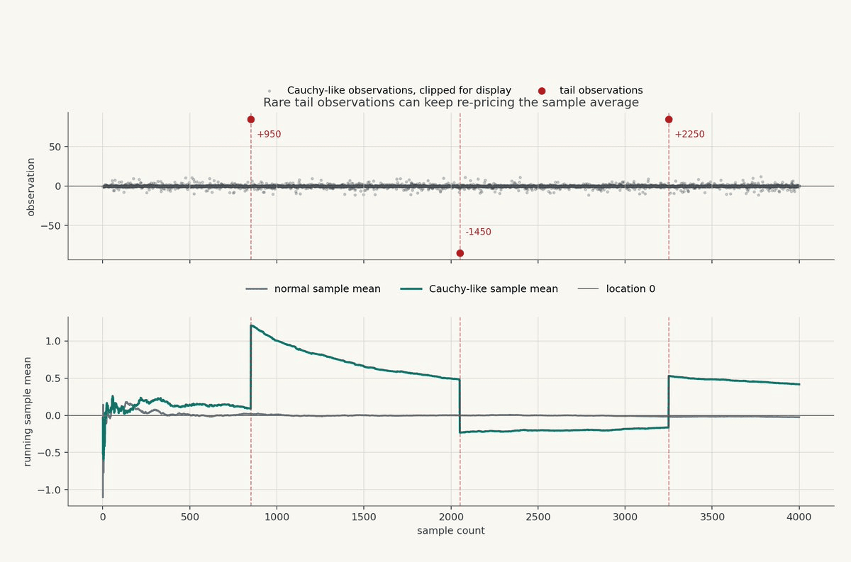
The graph is synthetic, but the mechanism is the one that matters. The normal sample mean quickly compresses toward the reference level, while the Cauchy-like sample mean looks as if it is stabilizing until a single tail observation changes the estimate. A risk control that treats the current sample average as a stable state variable would be interpreting a temporary quiet period as convergence, when the process has not actually granted the estimator that right.

Tail Events Are State Transitions

The average row in a backtest describes a regime in which the market system is still behaving close enough to the assumptions under which the strategy was designed, whereas tail observations describe regimes in which those assumptions become endogenous to the stress itself. A directional signal that maps cleanly into a target position during ordinary liquidity conditions may become a different object when slippage, latency, funding, book depth, venue reliability, liquidation thresholds, and the probability of correlated de-risking are all moving against the strategy at once.

Nassim Taleb's turkey example is useful here not as a colorful story about surprise, but as a compact description of a missing state variable. For readers unfamiliar with it, Taleb describes a turkey that is fed every day and therefore appears to have increasing evidence that humans are benevolent, right up until the Thanksgiving state change invalidates the entire model.The turkey's ordinary observations do not estimate the bad state poorly; they fail to represent it at all, and many trading strategies inherit the same shape when thousands of ordinary observations reinforce a regime classification that breaks exactly when the market changes state.

The more structural risk question, therefore, is not only how large the next loss might be, but what market-state transition would make the strategy's current target-position policy invalid.

The Normal Model Compresses State Into Scale

The Gaussian model is attractive because it compresses uncertainty into a center and a scale:

For many local calculations this compression is useful, since it creates a common coordinate system for deviations from ordinary behavior; notwithstanding that usefulness, it also tempts the researcher to treat unusual observations as scaled versions of the same state, so that a four-sigma move, a six-sigma move, and a ten-sigma move differ only by magnitude while the underlying market mechanism is presumed constant.

Under a standard normal model, a six-sigma event is nearly absent:

When markets repeatedly produce observations that a model classifies as six sigma, the first hypothesis should not be that rare miracles are occurring with suspicious frequency, but that the randomness has been specified incorrectly. The process may be drawn from a fat-tailed distribution, a mixture of regimes, a jump process, a liquidity-constrained market, or a network of positions whose forced flows are invisible to a normal model but decisive for realized loss.

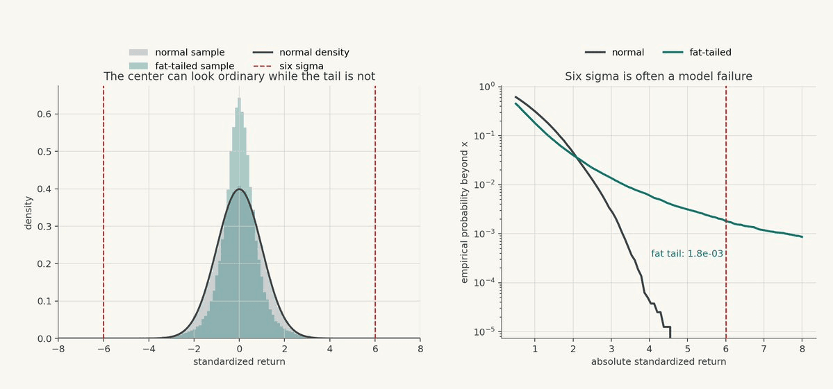
The synthetic example shows why this failure is easy to miss. Near the center, the normal and fat-tailed samples can look similar enough to satisfy casual diagnostics; in the tail, the distributional error becomes the object that controls strategy survival.

Fat Tails Are A Statement About Decay

A fat-tailed distribution assigns more probability to extreme outcomes than a thin-tailed distribution, but the more useful statement for strategy design is that tail shape governs the rate at which extreme outcomes become irrelevant. Volatility is a scale parameter; tail shape is a decay law; confusing the two lets a strategy appear measured while leaving its ruin profile mostly unmodeled.

The coarse taxonomy is sufficient for most trading design work:

• Gaussian-like tails decay extremely fast, with all moments finite.

• Exponential-like tails decay more slowly than Gaussian tails, but still impose a relatively fast penalty on extremes.

• Power-law tails decay polynomially, allowing remote outcomes to remain operationally material.

A common power-law form is:

The tail index alpha governs moment existence:

When alpha is less than or equal to 2, the variance of the idealized distribution is not finite; when alpha is less than or equal to 1, even the mean is not finite. A live strategy operates in finite samples and finite markets, so the operational implication is not a metaphysical argument about infinity, but the simpler and more dangerous fact that estimates become unstable, a small number of paths can dominate the result, and conventional moment-based controls can remain calm while the actual strategy is approaching a state it cannot afford.

Finance has produced serious examples of this problem. In Mandelbrot's 1963 paper on speculative prices, cotton price changes were modeled with stable Paretian laws rather than Gaussian laws; under a stable law with tail index below 2, the model has no finite second moment, which means the variance is not a population quantity waiting to be estimated more carefully. The practical implication is severe: if the process is closer to that model than to Brownian motion, then a volatility estimate may be a useful local statistic without being a stable description of the loss-generating mechanism.

Markets contain mechanisms that naturally produce this behavior: discontinuous repricing, liquidation cascades, crowded exits, fragmented liquidity, stale marks, collateral thresholds, volatility clustering, and sudden changes in venue capacity. Crypto adds additional state variables, including oracle mechanics, on-chain congestion, permissionless venue liquidity, smart contract risk, and technical failures that may not appear in historical returns until they matter.

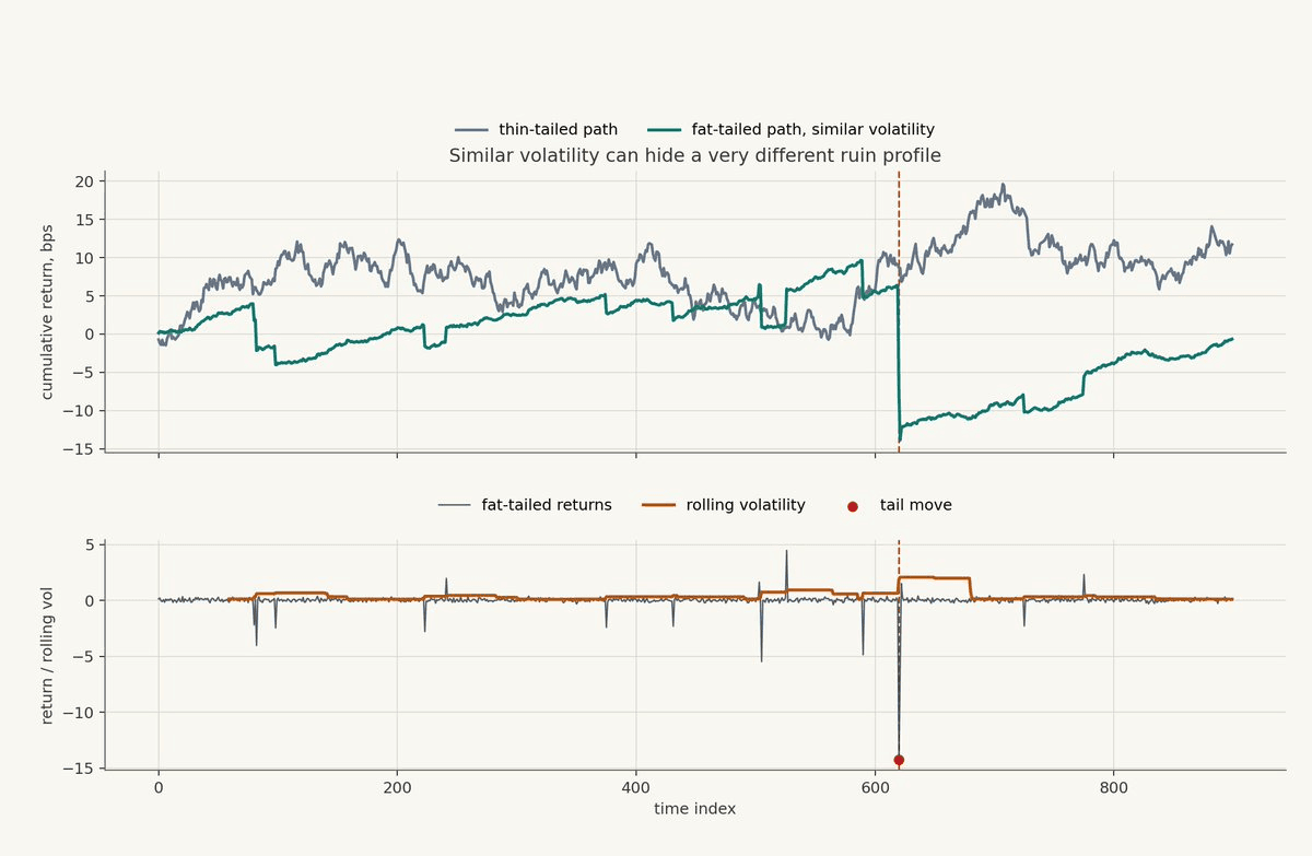
Holding realized volatility roughly constant while changing the tail mechanism produces two paths that can look comparable in a summary table and radically different under a survival constraint. In the lower panel, the red marker is the kind of observation a thin-tail model would treat as essentially unavailable, yet the total realized volatility of the path can still be engineered to resemble the thin-tailed path by making the rest of the process quieter. The table is not necessarily wrong; it is answering a thinner question than the strategy needs answered, because it has collapsed path shape, jump concentration, and recovery burden into one scale number.

Volatility Is An Estimator, Not A Tail Model

A causal volatility estimate remains a useful component of the strategy machinery, especially for normalization, regime classification, and target-position scaling. One common exponentially weighted estimator is:

Here, tau is a practitioner-chosen memory parameter, with shorter values increasing responsiveness and noise and longer values increasing stability and lag.

As an estimator of recent squared-return scale, this object is coherent; as a representation of tail state, it is structurally incomplete. It does not distinguish continuous high volatility from jump risk, symmetric dispersion from downside skew, ordinary turnover from forced liquidation, or a wide-but-tradable spread from a market in which the book disappears before the strategy can move its achieved exposure toward its target.

Consequently, volatility can be an input to a state machine, a normalization parameter, or a target-position constraint, but it should not be treated as the state machine itself.

VaR Marks A Boundary; ES Measures The Interior

Let L denote loss. Value at Risk defines a boundary at confidence level alpha:

Expected shortfall defines the conditional average loss after that boundary has been crossed:

VaR identifies the quantile at which the system enters the tail, whereas ES measures the interior of that tail, where ordinary observations have stopped carrying most of the information relevant to survival. For target-position design, the interior often matters more than the boundary, because two strategies with similar VaR can impose very different collateral, drawdown, liquidity, and operational demands once the threshold is breached.

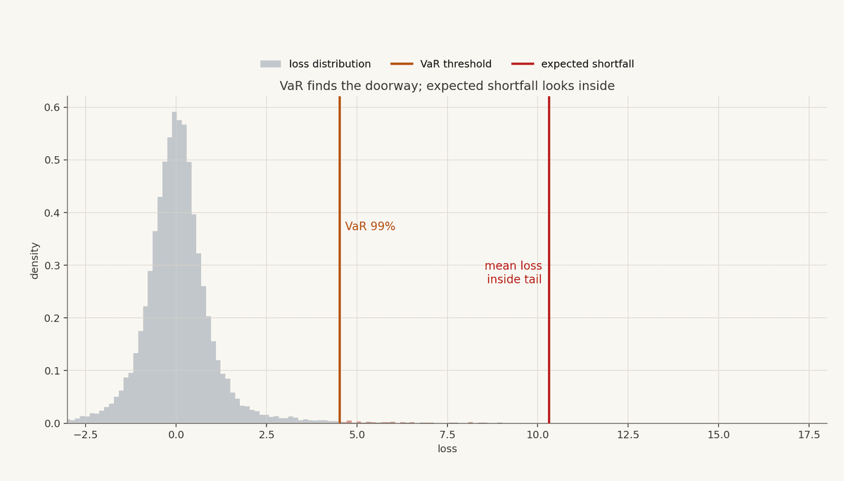
A strategy capped only by a VaR threshold can still be too large if the conditional loss beyond that threshold consumes the available error budget faster than the state machine can reduce exposure.

EVT Treats The Tail As Its Own Object

Extreme value theory changes the assignment of modeling effort by refusing to make the center of the distribution explain the region where the strategy is most likely to fail. Rather than fit one comfortable distribution to both ordinary returns and extreme losses, EVT isolates the tail as its own estimation problem.

Two constructions are common:

• "Block maxima" model the largest observation in each block.

• "Peaks over threshold" model observations beyond a high threshold.

For trading systems, peaks over threshold often maps more naturally onto control logic, because a strategy can observe losses L, choose a threshold u, and study the exceedance above that threshold:

Under broad regularity conditions, exceedances over a sufficiently high threshold can be approximated by the generalized Pareto distribution:

The parameter u is the threshold, Y is the exceedance, beta is the tail scale, and xi is the tail shape; these quantities are useful not because they decorate the distribution with more notation, but because they become possible control surfaces for target-position caps, pause states, cooldowns, and unknown-regime logic.

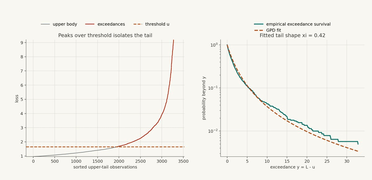
The left panel is sorted loss space, not time. The gray line is the upper body of the loss distribution, the orange dashed line is the threshold u, and the red segment is the set of observations the model has decided to treat as tail exceedances. The right panel then discards the body and asks a narrower question on log scale: conditional on already being beyond u, how quickly does the probability of even larger exceedances decay? The distance between the empirical survival curve and the fitted GPD is therefore not a cosmetic fit error; it is evidence about whether the chosen threshold and tail family are plausible enough to become strategy controls.

The construction does not make the whole distribution elegant. It assigns modeling attention to the part of the distribution where the strategy's assumptions are most likely to become false.

The Tail Shape Parameter Controls The Far State

The parameter xi determines the qualitative behavior of the fitted tail:

• xi < 0: bounded tail

• xi = 0: exponential-like tail

• xi > 0: heavy tail

When xi > 0, remote losses decay slowly enough to remain operationally relevant, which means the far state is no longer merely a theoretical limit but a regime that can determine allowable inventory, target-position size, turnover limits, and whether the strategy should be permitted to express a signal at all.

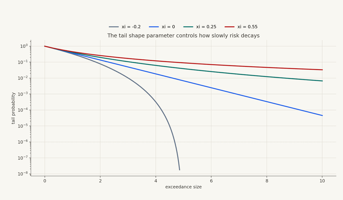
The estimate should be treated with suspicion, since tail samples are few by construction, a few observations can move xi, and venue mechanics can change the loss process without asking the estimator for permission. Notwithstanding those limitations, an explicit tail-shape estimate is still superior to an implicit Gaussian tail buried inside a volatility number, because the assumption has been made visible enough to challenge.

Threshold Selection Is Model Governance

The threshold u is not a technical nuisance but a governance decision over what the model is allowed to call the tail. If u is too low, ordinary observations contaminate the exceedance distribution and the estimator becomes a hybrid of body and tail; if u is too high, too few observations remain and the estimator becomes unstable. The threshold therefore allocates error between bias and variance while also encoding a market judgment about when the loss process has entered a different state.

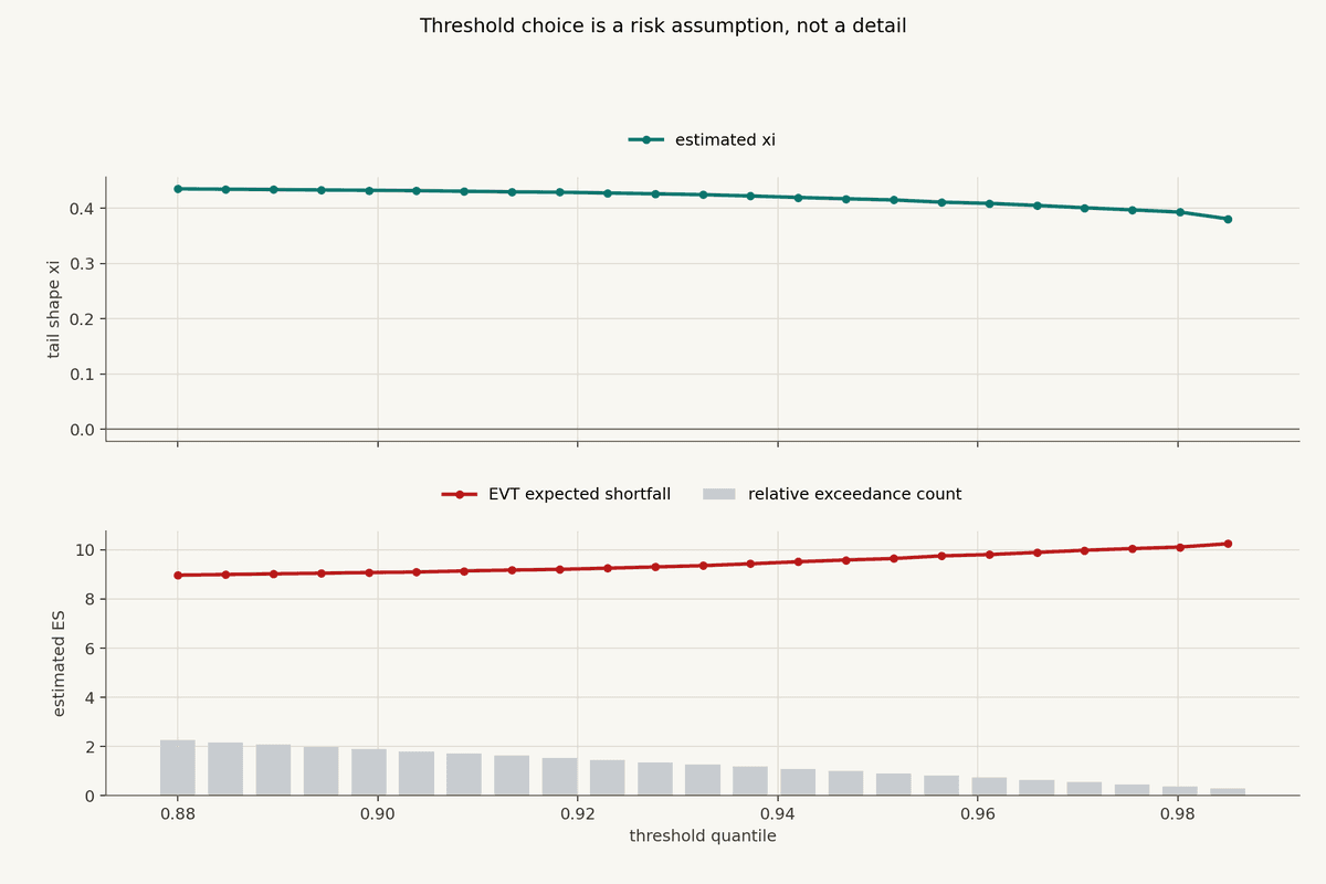
The top panel shows how the estimated tail-shape parameter xi changes as the threshold quantile moves upward. The lower panel shows the corresponding expected shortfall estimate, while the gray bars show the relative number of exceedances left to fit. Moving right makes the threshold more selective, so the model is using purer tail observations but fewer of them; moving left gives the estimator more data, but risks contaminating the tail with ordinary losses. A usable threshold region is not one magic point, but an interval where xi, ES, exceedance count, and market intuition do not contradict each other.

The workflow should inspect exceedance counts, tail-shape stability, expected-shortfall sensitivity, and the market mechanism that produced the observations. A threshold that looks statistically convenient while cutting across a real liquidity, spread, liquidation, or execution-cost boundary is usually less meaningful than a threshold that corresponds to a recognizable market-state transition, even if the latter leaves the estimator less cosmetically smooth.

Tail Estimation Becomes Strategy Logic

Once a tail estimator is causal, it can enter the strategy as a constraint rather than remain a statistic observed after the fact. Suppose the strategy would otherwise emit target position q_t; a tail-aware policy can cap the allowable target as estimated expected shortfall rises:

The function h is a decreasing assignment from estimated tail loss to allowable exposure, so that a larger conditional loss estimate produces a smaller target-position budget. The same estimator can define a state transition:

In this form, an estimate becomes a constraint, and the constraint becomes either a state transition or a target-position cap. Tail risk has entered deterministic strategy logic.

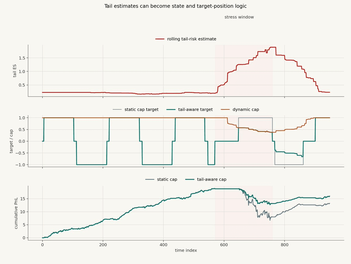
The top panel is the causal tail-risk estimate computed through time; it rises only after the loss process begins producing observations that belong to the stress state. The middle panel shows the operational consequence: the static strategy continues to ask for the same target position, while the tail-aware strategy multiplies that target by a dynamic cap that contracts as estimated ES rises. The lower panel is not meant to claim that this particular synthetic rule is optimal; it shows the behavioral difference between a risk estimate that only gets plotted and a risk estimate that is allowed to change the target position.

Structure's architecture is built around exactly this kind of separation. A strategy turns tick-level data into deterministic signals; signal values determine state and state transitions through simple control flow; each state resolves to target positions; and the target executor manages orders to achieve those target positions outside the strategy logic. If a tail estimate changes the state or the target position, the change belongs inside the auditable logic of the strategy rather than in an informal risk instruction that sits outside the system.

Risk controls are not external to the strategy when they determine what the strategy is allowed to do.

Backtesting Tail Logic Requires Causality

EVT can leak like any other estimator, and the violation is especially tempting because the tail is easiest to describe after the stress period has already occurred. The invalid version fits the tail model on the full sample, observes the eventual stress regime, and gives the strategy a tail estimate it could not have had at the decision time.

A causal tail estimate has the form:

Here, Psi is the estimation procedure, and u_t is the threshold chosen using information available through time t; the backtest must therefore replay the full decision loop with the estimate available only after it would have been computed.

The relevant comparison is behavioral rather than cosmetic: static caps versus tail-aware caps, normal VaR versus EVT VaR, normal ES versus EVT ES, strategies with and without pause states, sensitivity across thresholds, and performance through known stress windows without allowing those windows to train the control before they occur. At trading firms, many attractive risk overlays die here because they explain the crisis after the fact but do not change the strategy early enough when replayed causally; the backtest has not failed, it has exposed an estimator that describes the tail later than the strategy needs to act.

Historical Mechanisms, Not Morals

Long-Term Capital Management is often flattened into a morality play about leverage, although the more useful mechanism is path dependence: many of the fund's trades had a coherent convergence thesis, yet the path to convergence passed through widening spreads, crowded positions, financing pressure, and counterparties that did not have to wait for theoretical value to arrive. The trade could be conceptually reasonable and still become impossible to finance.

The March 2020 Treasury market stress carries the same structural lesson in a market usually treated as deep and liquid. When many participants wanted cash at once and dealer balance sheets were constrained, liquidity was no longer a background constant but a state variable; a risk model that treated Treasury liquidity as invariant was not merely underestimating volatility, but representing the wrong market system.

Crypto liquidation cascades make the mechanism even more explicit: price movement weakens collateral, weakened collateral triggers forced selling, forced selling moves price, and the loop propagates across accounts and venues. In that regime, a return observation is also evidence about a network state composed of collateral buffers, liquidation thresholds, book depth, venue health, and the probability of additional forced flow.

These episodes are not useful because they provide atmosphere but because they exhibit the same invariant: tail losses often arise when price movement, liquidity, funding, positioning, and operations become one coupled system.

EVT Does Not Make The Tail Obedient

EVT makes the tail explicit without making it stable, stationary, or obedient to the estimator. The remaining constraints are not small:

• Tail samples are few.

• Threshold selection is unstable.

• Observations are dependent.

• Volatility clusters.

• Market structure changes.

• Crowded strategies feed back into price.

• Venue mechanics can dominate the return history.

• Crypto execution, oracle, liquidity, and technical risks may be absent from the sample until they matter.

These limitations prevent EVT from becoming theology, which is exactly why the framework is useful. It gives the strategy designer a disciplined way to express tail assumptions, test sensitivity, and convert tail-state information into auditable behavior without pretending that the estimator is managing the tail.

The Strategy Contains The Tail It Assumes

Consider a strategy whose state machine, signal vector, and parameter set resolve to a target-position function:

If there is no tail-state variable in this assignment, then the strategy has not avoided a tail model; it has adopted one in which the current state s_t and feature vector x_t remain sufficient even when liquidity, collateral, spread, funding, and executable size have changed their relationship to one another. This is a strong assumption, and in many markets it is the wrong one.

A tail-aware strategy instead admits another object into the assignment:

Here, z_t can be an EVT estimate, an expected shortfall estimate, a threshold-exceedance state, or a broader unknown-regime indicator. The particular estimator matters, but the structural change matters more: tail information is no longer commentary on the strategy after the fact; it is one of the quantities by which the strategy determines what operation it is allowed to perform.

Accordingly, the purpose of fat-tail modeling is not to produce a more impressive risk limit. It is to promote otherwise hidden assumptions into explicit objects: thresholds, exceedances, shape parameters, expected shortfall estimates, target-position caps, pause states, and causal backtests. Once promoted, these objects can be inspected, versioned, rejected, or made part of deterministic execution logic.

For production-grade trading algos, this is the standard worth insisting on: the strategy's risk assumptions should be visible in the machinery of the strategy itself, not appended as prose after the state machine and target positions have already been chosen.

Not Financial Advice

The content above is for general educational and informational purposes only. It is not financial, investment, trading, legal, tax, accounting, or other professional advice, and it is not a recommendation, offer, or solicitation to buy, sell, hold, or use any asset, strategy, protocol, venue, or financial product.

Trading and automated strategies involve substantial risk, including the possible loss of principal. Crypto assets and DeFi markets can be highly volatile, illiquid, technically complex, and subject to execution, smart contract, custody, regulatory, and counterparty risks. Past performance, backtests, simulations, or examples do not guarantee future results.

You are responsible for your own decisions. Do your own research, understand the risks, and consult qualified professional advisers before making financial, legal, tax, or trading decisions. Structure does not provide personalized investment advice and does not guarantee any strategy outcome, return, or level of performance.