This article follows our post on Limit Order Book Transformers

Time-series foundation models are arriving in finance with a familiar promise: pretrain once, adapt many times. I think the promise is worth taking seriously, but only if we are precise about what is supposed to transfer.

The useful version of the claim is narrow. A pretrained time-series model may learn recurring temporal structure - persistence, shock response, regime shifts, lead-lag behavior, volatility clustering, etc. - before we ask it to solve a specific trading problem. If that representation transfers, the local research job becomes easier: less clean data may be needed to calibrate a forecast, detect a regime, or estimate a state variable.

The hard part is that financial time series are produced by market mechanisms, not by a neutral sequence generator. Quotes, trades, funding, liquidity, positioning, collateral constraints, and other models in the same market all help produce the observations. A model can learn a useful temporal pattern and still be wrong about its economic meaning, because the same shape can map to very different payoffs depending on venue, horizon, costs, crowding, and regime.

This post treats time-series foundation models as candidate representation engines and forecasters. The question is whether they improve the research loop after causal validation, calibration, cost-aware backtesting, regime controls, and target-position logic have all had their say.

What A Time-Series Foundation Model Is

A time-series foundation model is pretrained across many sequences so it can be reused on downstream time-series tasks: forecasting, classification, anomaly detection, imputation, regime detection, representation extraction, etc.

The simplest forecasting form is:

The symbols are less important than the separation. The model receives the historical context window available at decision time and the requested forecast horizon, then emits a forecast for the future target. The parameter set phi comes from broad pretraining rather than from the specific trading strategy alone.

Fine-tuning adds task-specific calibration:

The pretrained parameters carry the broad temporal representation. The task-specific parameters learn the local mapping for the particular asset, venue, frequency, label, or forecasting objective.

Three uses tend to get mixed together:

• zero-shot forecasting: use the pretrained model on a new series without fitting it to that series

• fine-tuning: adapt the model to the target task, market, or label

• representation extraction: use the model's hidden state as an input to another model or state machine

Zero-shot forecasting means the model is asked to forecast a target series without additional training on that specific target series. In a research workflow, that can be a useful first pass. In a live trading workflow, it is only a starting point.

What Might Transfer

At a trading firm, the first practical question is whether the model has learned shapes that a trader or researcher would already recognize as reusable.

Volatility clusters. Shocks decay. Liquidity widens and refills. Related instruments sometimes lead or lag each other for a few ticks before the relationship disappears. Those patterns do not define a strategy, but they do define temporal structure that can appear across assets, venues, and frequencies.

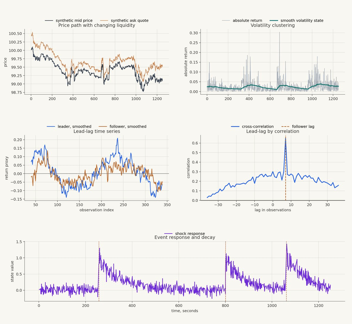
This figure is synthetic, but each panel is meant to isolate a kind of reusable temporal structure.

The top-left panel shows a synthetic mid price and a synthetic ask quote. The vertical distance between them is an illustrative spread/liquidity state: when the quote moves farther from the mid, the market is effectively more expensive to trade in this toy example. The price path is not the object of interest; the joint movement of price and liquidity state is.

The top-right panel shows volatility clustering. The gray series is the absolute return at each observation, while the green line is a smoothed volatility state. Markets often move this way: large moves are not evenly scattered through time, and the local variance process has memory.

The middle-left panel shows the lead-lag relationship in the raw synthetic series. The orange follower series responds after the blue leader series, which is the kind of delayed relationship that can be easy to miss when each series is noisy on its own.

The middle-right panel measures the same relationship by lagged cross-correlation. The peak near the dashed vertical line means the follower contains the strongest information about the leader after that delay. This is useful because lead-lag structure is a temporal primitive: it tells the model that the relationship is not only between two values, but between two values separated by a specific amount of market time.

The bottom panel shows event response and decay. A shock enters the system, the state jumps, and then the effect decays rather than disappearing immediately. That shape shows up in many places: spread normalization after a volatility burst, volume after a news event, funding pressure after a crowded move, etc.

A foundation model that has seen many variants of these structures may need fewer local examples to recognize a related pattern. The remaining question is economic: what does the pattern mean for this target, on this horizon, under these costs?

Why Time Series Are Not Language

The language-model analogy is useful, but it breaks if we forget what the objects are. Text models operate on tokens whose role is often stable enough to transfer across documents. Time-series models operate on measurements whose meaning depends on scale, sampling scheme, units, venue mechanics, and regime. A return, a spread, and a top-of-book size series may all be sequences, but they are produced by different market operations.

A one-second return forecast, a one-hour volatility forecast, and a one-week inventory forecast are not interchangeable merely because the model interface can ask for a horizon. In markets, there is also feedback: when enough capital reacts to similar forecasts, the forecast becomes part of the state it is trying to predict.

This suggests a few design hypotheses for finance, if we may be so bold:

First, normalization and tokenization should respect economic meaning. Prices, returns, spreads, depth, and funding should not be treated as interchangeable numeric streams just because they can be patched into the same transformer.

Second, event time may matter as much as clock time. Some processes evolve through trades, quote updates, auctions, liquidations, or funding events rather than through evenly spaced timestamps. The "market time" concept enters here.

Third, distributional forecasts are often more useful than point forecasts. A forecast that says the next state is uncertain, fat-tailed, or outside the training region may be more valuable than a confident conditional mean.

Fourth, out-of-domain state should be explicit. In production, "unknown regime" is a useful (and mature) trading state; it can reduce size, widen thresholds, or stop trading all together.

The Current Model Families

The field is moving quickly, but a few model families are useful reference points.

Google's TimesFM is a decoder-only transformer trained for time series forecasting. A decoder is a causal transformer block: it reads past context and predicts future values without looking ahead into the future part of the sequence. TimesFM groups contiguous observations into patches, which lets the model process and forecast chunks of time rather than one point at a time. Source: https://research.google/blog/a-decoder-only-foundation-model-for-time-series-forecasting/

Amazon's Chronos takes a different route. It scales and quantizes time-series values into a finite vocabulary, then trains transformer language-model architectures with cross-entropy, closer to the way text models predict tokens. That design makes the language analogy explicit while still leaving the hard finance questions - scale, units, target semantics, trading costs - to the user. Source: https://www.amazon.science/publications/chronos-learning-the-language-of-time-series

Moirai emphasizes universal forecasting across frequencies, variable counts, and heterogeneous datasets. Its LOTSA training corpus was built to cover many domains and billions of observations, which makes it a useful example of the "many time series, many mechanisms" approach rather than a single-domain forecasting model. Source: https://arxiv.org/abs/2402.02592

MOMENT is useful because it frames the problem beyond point forecasting. Representation learning, imputation, anomaly detection, and classification can matter just as much as the next forecast value when the model output becomes one input to a larger strategy process. Source: https://arxiv.org/abs/2402.03885

TinyTimeMixer, or TTM, pushes on a practical production question: how much transfer can you get from a smaller pretrained model? In trading, a model that is cheap to retrain, replay, monitor, and deploy can be more useful than a larger model with a cleaner benchmark table and worse operational properties. Source: https://research.ibm.com/publications/tiny-time-mixers-ttms-fast-pre-trained-models-for-enhanced-zerofew-shot-forecasting-of-multivariate-time-series--1

The skeptical papers are worth reading alongside the model papers, too. One recent critique argues that zero-shot performance depends heavily on pretraining domains, and that larger models do not automatically dominate smaller specialized models once memory, parameter count, and target similarity are considered. Source: https://arxiv.org/abs/2510.00742

Finance-specific work is more mixed, which is what you should expect. Some results report sample-efficiency gains from models like TTM and Chronos on multivariate financial forecasting tasks; other comparisons find that specialized models can still match or beat them. For a practitioner, the mixed result is the useful part: it shows where the pretrained representation is buying sample efficiency and where the local model still owns the problem. Source: https://arxiv.org/abs/2507.07296

Zero-Shot Is A Baseline, Then Comes Fine-Tuning

Zero-shot forecasting is attractive because it is fast. You give the model a context window from a new series, ask for a horizon, and get a forecast without fitting on that target series. In research, that gives you a quick baseline and sometimes a useful prior.

The serious question starts after that. Does the pretrained representation reduce the amount of local data needed to learn the target? Does fine-tuning adapt when the local mapping changes? Does the model know when the current input is outside the region where its forecast should be trusted?

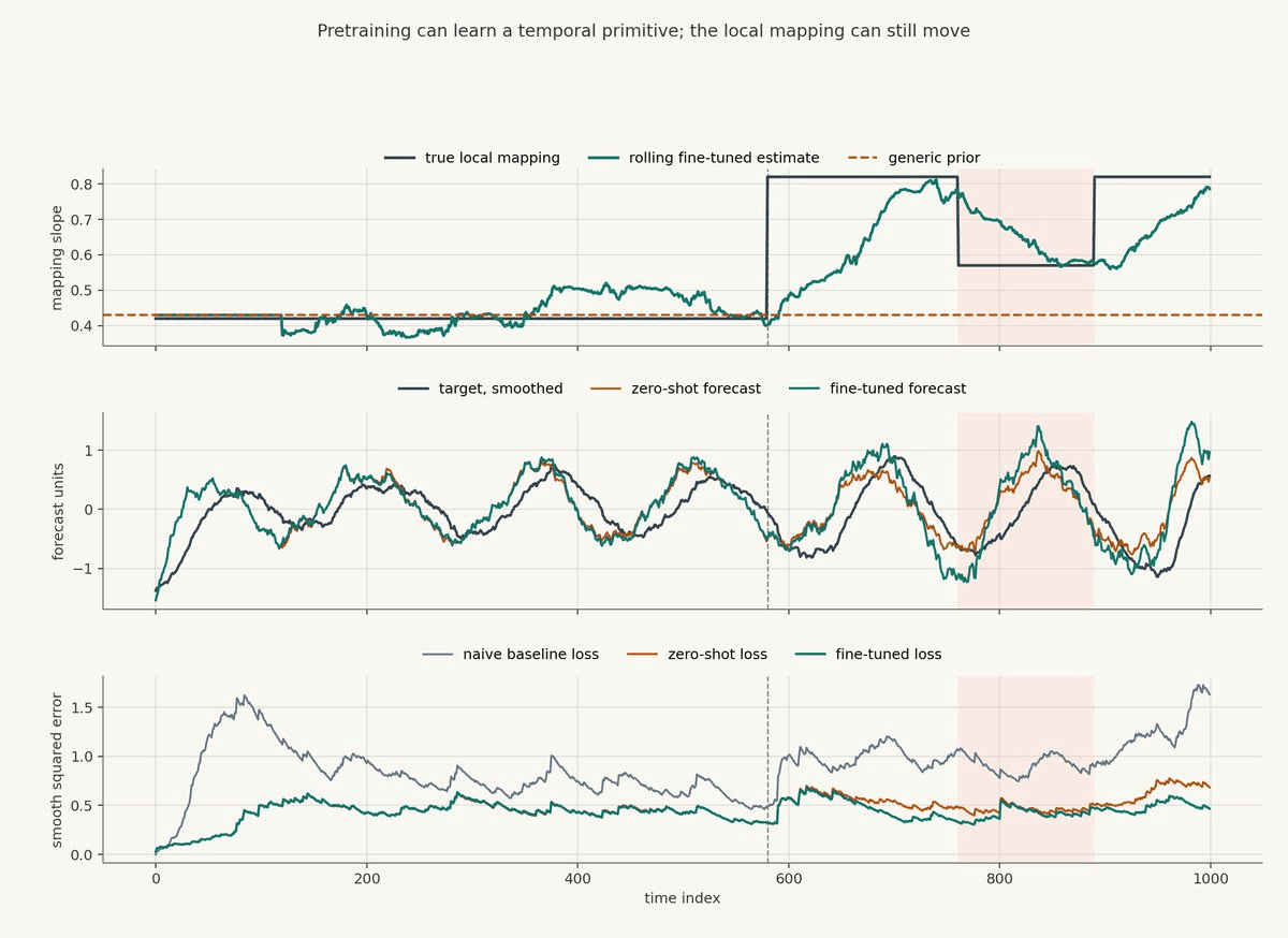
This chart is also synthetic. It was generated from a hidden temporal signal whose relationship to the future target changes over time.

The top panel shows the local mapping from temporal signal to target. The dark line is the true mapping used to generate the data. The orange dashed line is the generic prior, meant to stand in for a zero-shot model that has learned a reasonable average relationship from pretraining. The green line is a rolling fine-tuned estimate. It adapts, but not instantly; it has lag because it is only allowed to learn from recent history.

The middle panel shows the target, smoothed, against the two forecasts. Before the vertical dashed line, the generic prior is roughly acceptable. After the mapping changes, the zero-shot forecast keeps using the old slope, while the fine-tuned forecast moves closer to the new relationship. In the red shaded region, the mapping itself becomes less reliable, which is the kind of condition a live system should treat as an unknown state rather than as a normal forecast window.

The bottom panel shows smoothed squared error. The fine-tuned version is not perfect, but it generally controls error better once the local relationship moves away from the generic prior. Fine-tuning is valuable here because it lets a reusable representation be recalibrated to the current market rather than frozen at its average pretraining relationship.

In real research, the local mapping might be a relationship between spread state and next-minute volatility, queue imbalance and short-horizon mid-price movement, funding pressure and cross-asset returns, or volume rhythm and expected slippage. The shape learned during pretraining can help, but the mapping from shape to payoff has to be learned locally.

The Best Use Case May Not Be Raw Price Direction

The obvious question is whether a foundation model can predict the next return. Sometimes that is the right target, but it is often the most challenging one: low signal-to-noise, crowded, adaptive, and expensive to monetize after costs.

The more useful targets may sit one layer upstream from direction: volatility, liquidity, volume, fill probability, slippage, regime state, missing-data repair, anomaly detection, etc. These variables matter because they change how much exposure a strategy should take, whether it should trade at all, and how much confidence it should place in a directional signal.

A volatility forecast can shrink the target-position cap before the strategy enters a high-variance state. A liquidity forecast can move the state machine from active to reduced when costs widen. A fill-probability forecast can suppress a signal that looks attractive on mid-price but is unlikely to be executable. An out-of-domain score can move the strategy into an unknown state where target positions are cut or forced flat.

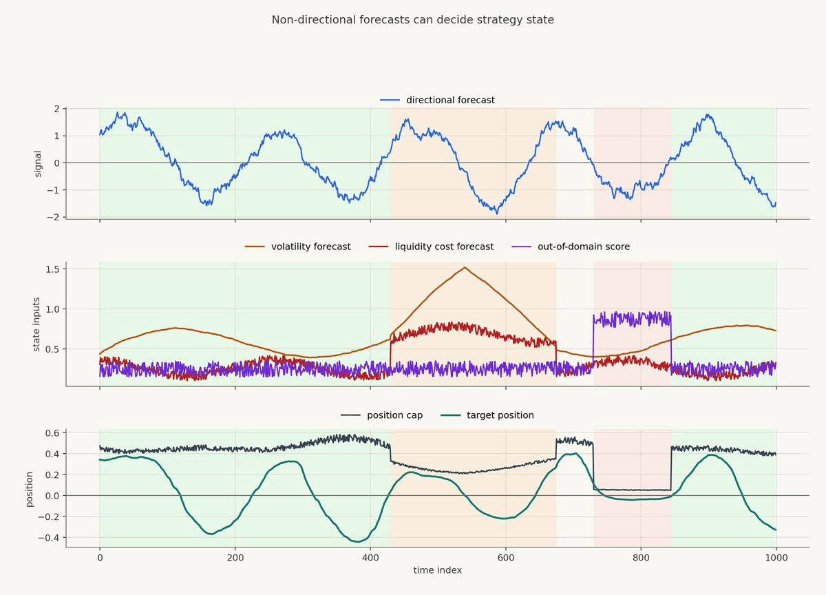
This figure shows one way to make that concrete.

The top panel is a synthetic directional forecast. If this were the only input, the strategy would simply move exposure up and down with the signal.

The middle panel adds three non-directional forecasts: volatility, liquidity cost, and an out-of-domain score. The orange shaded region is a reduced state caused by higher volatility and worse liquidity. The red shaded region is an unknown state caused by the out-of-domain score.

The bottom panel shows what happens to target position. The dark line is the position cap. The green line is the actual target position after the directional forecast has been passed through the cap and smoothed. During the reduced state, the cap falls even though the directional signal is still moving. During the unknown state, the cap is cut much harder.

One simple construction looks like this:

If the out-of-domain score is high, the cap can be reduced further:

The target position can then be formed by applying the directional signal to the current cap:

A better volatility or liquidity model may never forecast "up" or "down," but it can still improve the strategy by changing the state in which the directional forecast is allowed to express itself.

Evaluation Has To Be Harsher Than The Benchmark

Benchmark tables answer a narrow question: does one forecast model beat another on a dataset under a particular metric? A trading team needs to know whether the model improves the strategy after time-aware validation, calibration, costs, capacity, latency, and replay.

The evaluation should use forward time splits, not random row splits. If labels overlap, purge and embargo neighboring observations. Scaling and normalization should be fit only on training data or computed causally. The model should be compared against naive forecasts, linear models, tree models, and domain-specific baselines. Results should be broken down by horizon, regime, asset, venue, and volatility state instead of collapsed into one flattering number.

The most useful comparison is incremental utility:

The challenger matters only if the target positions it produces, after costs and out-of-sample replay, improve the strategy relative to the baseline. If it improves mean squared error while increasing turnover, worsening tail exposure, or concentrating all gains in one regime, the benchmark result has not earned much.

The deployment questions belong in the evaluation, too. Can the model be replayed deterministically? How often does it need to be fine-tuned? What data is allowed into the fine-tuning window? What happens when the input is stale, missing, or outside the training distribution? What state transition occurs when uncertainty is high?

For a trading system, those questions are part of the model's economic meaning.

How This Maps Into Structure

In Structure terms, a time-series foundation model belongs in the data, computations, and signals layer. It can consume tick-level data and other time-series inputs, compute a learned representation, and emit a forecast, uncertainty score, regime embedding, or state variable.

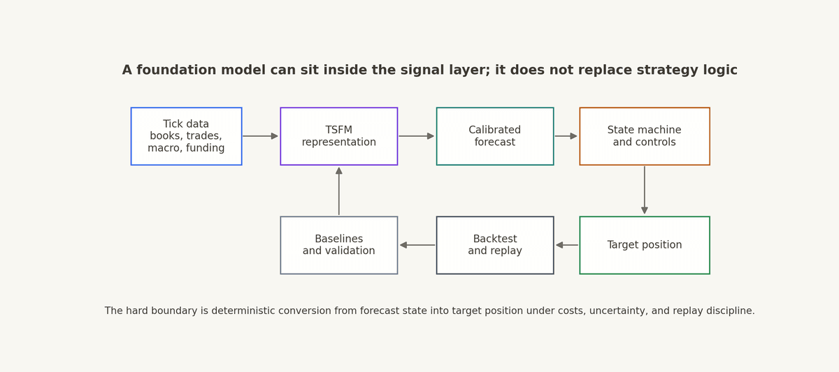
The separation can be written as:

The first line turns recent data history into a learned representation. The second line turns that representation, together with current cost and execution state, into a calibrated forecast. The third line turns strategy state, forecast, costs, uncertainty, and parameters into a target position.

That boundary is important. The model can improve the signal layer, but the strategy still needs auditable logic that decides when the signal is active, stale, contradicted by costs, outside its training domain, or too uncertain to trade. The output of the strategy is the target position; execution sits outside the strategy logic.

What To Watch

I would watch the papers that make domain shift, uncertainty, and fine-tuning part of the main result rather than a footnote. Lower forecast error is useful, but in trading the more interesting result is transfer across regimes with clean time splits, strong baselines, causal preprocessing, and a believable story for how the forecast becomes position state.

The likely near-term use is a pretrained temporal representation feeding smaller local models, state estimators, and regime controls. If the representation makes the research stack faster, improves sample efficiency, or gives better state variables for the strategy logic, it has earned a place in the toolkit.

Pretraining does not simplify the market mechanism. It can still make the genuinely reusable parts of the research process cheaper to initialize, run, and test.

Not Financial Advice

The content above is for general educational and informational purposes only. It is not financial, investment, trading, legal, tax, accounting, or other professional advice, and it is not a recommendation, offer, or solicitation to buy, sell, hold, or use any asset, strategy, protocol, venue, or financial product.

Trading and automated strategies involve substantial risk, including the possible loss of principal. Crypto assets and DeFi markets can be highly volatile, illiquid, technically complex, and subject to execution, smart contract, custody, regulatory, and counterparty risks. Past performance, backtests, simulations, or examples do not guarantee future results.

You are responsible for your own decisions. Do your own research, understand the risks, and consult qualified professional advisers before making financial, legal, tax, or trading decisions. Structure does not provide personalized investment advice and does not guarantee any strategy outcome, return, or level of performance.